Analytics in Delhi- Rank Correlation-Part I

Spearman’s Rank-Order Correlation

This guide will tell you when you should use Spearman’s rank-order correlation to analyse your data, what assumptions you have to satisfy, how to calculate it, and how to report it. If you want to know how to run a Spearman correlation in SPSS, go to our guide here. If you want to calculate the correlation coefficient manually, we have a calculator you can use that also shows all the working out (here).

When should you use the Spearman’s rank-order correlation?

The Spearman’s rank-order correlation is the nonparametric version of the Pearson product-moment correlation. Spearman’s correlation coefficient, (, also signified by r_s) measures the strength of association between two ranked variables.

What are the assumptions of the test?

You need two variables that are either ordinal, interval or ratio (see our Types of Variable guide if you need clarification). Although you would normally hope to use a Pearson product-moment correlation on interval or ratio data, the Spearman correlation can be used when the assumptions of the Pearson correlation are markedly violated. A second assumption is that there is a monotonic relationship between your variables.

What is a monotonic relationship?

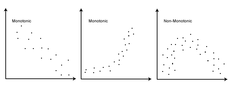
A monotonic relationship is a relationship that does one of the following: (1) as the value of one variable increases, so does the value of the other variable; or (2) as the value of one variable increases, the other variable value decreases. Examples of monotonic and non-monotonic relationships are presented in the diagram below (click image to enlarge):

 

Why is a monotonic relationship important to Spearman’s correlation?

A monotonic relationship is an important underlying assumption of the Spearman rank-order correlation. It is also important to recognize the assumption of a monotonic relationship is less restrictive than a linear relationship (an assumption that has to be met by the Pearson product-moment correlation). The middle image above illustrates this point well: A non-linear relationship exists, but the relationship is monotonic and is suitable for analysis by Spearman’s correlation, but not by Pearson’s correlation.

How to rank data?

In some cases your data might already be ranked, but often you will find that you need to rank the data yourself (or use SPSS to do it for you). Thankfully, ranking data is not a difficult task and is easily achieved by working through your data in a table. Let us consider the following example data regarding the marks achieved in a maths and English exam:

English	56	75	45	71	61	64	58	80	76	61
Maths	66	70	40	60	65	56	59	77	67	63

The procedure for ranking these scores is as follows:

First, create a table with four columns and label them as below:

English (mark)	Maths (mark)	Rank (English)	Rank (maths)
56	66	9	4
75	70	3	2
45	40	10	10
71	60	4	7
61	65	6.5	5
64	56	5	9
58	59	8	8
80	77	1	1
76	67	2	3
61	63	6.5	6

You need to rank the scores for maths and English separately. The score with the highest value should be labelled “1” and the lowest score should be labelled “10” (if your data set has more than 10 cases then the lowest score will be how many cases you have). Look carefully at the two individuals that scored 61 in the English exam (highlighted in bold). Notice their joint rank of 6.5. This is because when you have two identical values in the data (called a “tie”), you need to take the average of the ranks that they would have otherwise occupied. We do this as, in this example, we have no way of knowing which score should be put in rank 6 and which score should be ranked 7. Therefore, you will notice that the ranks of 6 and 7 do not exist for English. These two ranks have been averaged ((6 + 7)/2 = 6.5) and assigned to each of these “tied” scores.

What is the definition of Spearman’s rank-order correlation?

There are two methods to calculate Spearman’s rank-order correlation depending on whether: (1) your data does not have tied ranks or (2) your data has tied ranks. The formula for when there are no tied ranks is:

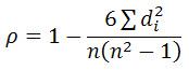
where d_i = difference in paired ranks and n = number of cases. The formula to use when there are tied ranks is:

where i = paired score.

—————————————————————To be  continued in our next post——————————————————————–

Related articles

• Basics of Statistical Analysis (traininginsas.wordpress.com)

Correlation in Analysis

Presentation for Correlation

Correlation

learn analytics in Delhi Statistical Analysis
learn SQL Server in Delhi Sql Server with SSIS,SSRS
learn SAS in Delhi Base SAS, Advance SAS

Basics of Statistical Analysis

When performing analysis to answer a research question, it is important to first identify the types of variables that will be used and choosing an outcome variable and one or more potential “independent” or determining variables. Once this is done, you must decide how you would like to use these in a statistical test to see if a relationship exists. The table below gives an idea of how to choose the appropriate test to use for statistical analysis depending on the variables you have chosen:

PREDICTOR VARIABLE (S)	OUTCOME VARIABLE
	Categorical	Continuous
Categorical	Chi Square, Log linear, Logistic	t-test, ANOVA (Analysis of Varirance), Linear regression
Continuous	Logistic regression	Linear regression,  Pearson correlation
Mixture of Categorical and Continuous	Logistic regression	Linear regression, Analysis of Covariance

Chi-Square –

Normally continuous outcome variables are used for anthropometry (e.g. wt/age z-score), but a categorical variable (e.g. malnourished yes/no for individual cases) is sometimes useful. For clinical signs, such as goitre, the data start as categorical variables. The chi-square test might be used any time the cross-tabulation function is used in SPSS. Chi-square is used to look at the statistical significance of an association between a categorical outcome (such as wasted or not wasted) and a categorical determining variable (such as diarrhea in the last two weeks, no diarrhea). When running the cross-tab, an option is available to test the significance of the association using chi-square. According to SPSS Version 8.0, Chi-Square (Crosstabs) Tests the hypothesis that the row and column variables are independent, without indicating strength or direction of the relationship. Pearson chi-square, likelihood-ratio chi-square, and linear-by-linear association chi-square are displayed. For 2×2 tables, Fisher’s exact test is computed when a table that does not result from missing rows or columns in a larger table has a cell with an expected frequency of less than 5. Yates’ corrected chi-square is computed for all other 2×2 tables.

ANOVA(Analysis of Variance)

ANOVA is used to see an association between a continuous outcome variable (such as mean HAZ score) and a categorical determining variable (such as iodized salt consumption). The ANOVA is an option under the SPSS 8.0 function Statistics, Compare Means, Means which runs the mean outcome variable in categorized groups. The ANOVA is a Statistics option under the Means function that allows for testing the difference between the mean outcome scores for the two or more categories of the determining variable. According to SPSS 8.0, Analysis of VarianceAnalysis of variance, or ANOVA, is a method of testing the null hypothesis that several group means are equal in the population, by comparing the sample variance estimated from the group means to that estimated within the groups.

One -way ANOVA– According to SPSS 8.0, The One-Way ANOVA procedure produces a one-way analysis of variance for a quantitative dependent variable by a single factor (independent) variable. Analysis of variance is used to test the hypothesis that several means are equal. This technique is an extension of the two-sample t test.

Two-way ANOVA (Analysis of Covariance using the GLM function)- According to SPSS 8.0, The GLM General Factorial procedure provides regression analysis and analysis of variance for one dependent variable by one or more factors and/or variables. The factor variables divide the population into groups. Using this General Linear Model procedure, you can test null hypotheses about the effects of other variables on the means of various groupings of a single dependent variable. You can investigate interactions between factors as well as the effects of individual factors, some of which may be random. In addition, the effects of covariates and covariate interactions with factors can be included. For regression analysis, the independent (predictor) variables are specified as covariates.

Linear Regression

Linear regression is used quite often in medical in order to preserve the continous nutrition outcome (often z-scores) and to test the relationship of this outcome with a combination of continuous and categorical determining variables (such as illness, feeding practices including breastfeeding, environmental influences, SES, and care practices among others). According to SPSS 8.0, Linear Regression estimates the coefficients of the linear equation, involving one or more independent variables, that best predict the value of the dependent variable. For example, you can try to predict a salesperson’s total yearly sales (the dependent variable) from independent variables such as age, education, and years of experience. Regression Coefficients. Estimates displays Regression coefficient B, standard error of B, standardized coefficient beta, t value for B, and two-tailed significance level of t. Confidence intervals displays 95% confidence intervals for each regression coefficient, or a covariance matrix. Model fit. The variables entered and removed from the model are listed, and the following goodness-of-fit statistics are displayed: multiple R, R2 and adjusted R2, standard error of the estimate, and an analysis-of-variance table.
R squared change. Displays changes in R**2 change, F change, and the significance of F change.

Pearson Correlation

Correlation testing usually runs a continuous outcome (such as weight for age z-score) against a continous determining variable (such as family income) to see if they have a linear relationship (positive, negative or none). This type of test will not tell the strength of the relationship between the variables, but will indicate the existence of the relationship. According to SPSS 8.0, The Bivariate Correlations procedure computes Pearson’s correlation coefficient, Spearman’s rho and Kendall’s tau-b with their significance levels. Correlations measure how variables or rank orders are related. Before calculating a correlation coefficient, screen your data for outliers (which can cause misleading results) and evidence of a linear relationship. Pearson’s correlation coefficient is a measure of linear association. Two variables can be perfectly related, but if the relationship is not linear, Pearson’s correlation coefficient is not an appropriate statistic for measuring their association.

T-Test

A t-test looks at the difference in means of a continuous variable between two groups. Remember that the null hypothesis Ho has no difference in the means (i.e., µ1= µ2) and the alternative hypothesis has a difference in the means. Remember that the p-value (significant at <0.05) is the probability that you would find the answer you have (i.e. the difference in means) given that the null hypothesis is true.

Categorical Variables in Regression

In statistics, a categorical variable is a variable that can take on one of a limited, and usually fixed, number of possible values. Categorical variables are often used to represent categorical data. In computer science and some branches of mathematics, categorical variables are referred to as enumerations or enumerated types. Commonly (though not in this article), the word level is used to refer to one of the possible values of a categorical variable.

A categorical variable that can take on exactly two values is termed a binary variable or dummy variable and is typically treated on its own as a special case. As a result, categorical variables are often assumed to contain, or at least potentially contain, three or more values. See the discussion below.

Examples of values that might be represented in a categorical variable:

• The blood type of a person: A, B, AB or O.
• The state that a resident of the United States lives in.
• The political party that a voter in a European country might vote for: Christian Democrat, Social Democrat, Green Party, etc.
• The type of a rock: igneous, sedimentary or metamorphic.
• The identity of a particular word (e.g., in a language model): One of V possible choices, for a vocabulary of size V.

For ease in statistical processing, categorical variables may be assigned numeric indices, e.g. 1 through K for a K-way categorical variable (i.e. a variable that can express exactly K possible values). In general, however, the numbers are arbitrary, and have no significance beyond simply providing a convenient label for a particular value. In other words, the values in a categorical variable exist on a nominal scale: they each represent a logically separate concept, cannot necessarily be meaningfully ordered, and cannot be otherwise manipulated as numbers could be. Instead, valid operations are equivalence, set membership, and other set-related operations.

As a result, the central tendency of a set of categorical variables is given by its mode; neither the mean nor the median can be defined. As an example, given a set of people, we can consider the set of categorical variables corresponding to their last names. We can consider operations such as equivalence (whether two people have the same last name), set membership (whether a person has a name in a given list), counting (how many people have a given last name), or finding the mode (which name occurs most often). However, we cannot meaningfully compute the “sum” of Smith + Johnson, or ask whether Smith is “less than” or “greater than” Johnson. As a result, we cannot meaningfully ask what the “average name” (the mean) or the “middle-most name” (the median) is in a set of names.

Note that this ignores the concept of alphabetical order, which is a property that is not inherent in the names themselves, but in the way we construct the labels. For example, if we write the names in Cyrillic and consider the Cyrillic ordering of letters, we might get a different result of evaluating “Smith < Johnson” than if we write the names in the standard Latin alphabet; and if we write the names in Chinese characters, we cannot meaningfully evaluate “Smith < Johnson” at all, because no consistent ordering is defined for such characters. However, if we do consider the names as written, e.g., in the Latin alphabet, and define an ordering corresponding to standard alphabetical order, then we have effectively converted them into ordinal variables defined on an ordinal scale.

Categorical random variables are normally described statistically by a categorical distribution, which allows an arbitrary K-way categorical variable to be expressed with separate probabilities specified for each of the K possible outcomes. Such multiple-category categorical variables are often analyzed using a multinomial distribution, which counts the frequency of each possible combination of numbers of occurrences of the various categories. Regression analysis on categorical outcomes is accomplished through multinomial logistic regression, multinomial probit or a related type of discrete choice model.

Categorical variables that have only two possible outcomes (e.g., “yes” vs. “no” or “success” vs. “failure”) are known as binary variables (or Bernoulli variables). Because of their importance, these variables are often considered a separate category, with a separate distribution (the Bernoulli distribution) and separate regression models (logistic regression, probit regression, etc.). As a result, the term “categorical variable” is often reserved for cases with 3 or more outcomes, sometimes termed a multi-way variable in opposition to a binary variable.

It is also possible to consider categorical variables where the number of categories is not fixed in advance. As an example, for a categorical variable describing a particular word, we might not know in advance the size of the vocabulary, and we would like to allow for the possibility of encountering words that we haven’t already seen. Standard statistical models, such as those involving the categorical distribution and multinomial logistic regression, assume that the number of categories is known in advance, and changing the number of categories on the fly is tricky. In such cases, more advanced techniques must be used. An example is the Dirichlet process, which falls in the realm of nonparametric statistics. In such a case, it is logically assumed that an infinite number of categories exist, but at any one time most of them (in fact, all but a finite number) have never been seen. All formulas are phrased in terms of the number of categories actually seen so far rather than the (infinite) total number of potential categories in existence, and methods are created for incremental updating of statistical distributions, including adding “new” categories.

Related articles

• Dummy variables (healthaffairsturkey.wordpress.com)

Analytics Training in Delhi

Methods of Qualitative Data Analysis

Interpretive Techniques

The simplest analysis of qualitative data is observer impression: Expert or bystander observers examine the data, interpret it via forming an impression and report their impression in a structured and sometimes (quasi-)quantitative form. This attempt to give structure to mere observation is referred to as “coding” and forms an important step beyond the mere observation.

Coding

Coding is an interpretive technique that seeks to both organize the data and provide a means to introduce the interpretations of it into certain quantitative methods.

Most coding requires the analyst to read the data and demarcate segments within it. Each segment is labeled with a “code” – usually a word or short phrase that suggests how the associated data segments inform the research objectives. When coding is complete, the analyst prepares reports via a mix of: summarizing the prevalence of codes, discussing similarities and differences in related codes across distinct original sources/contexts, or comparing the relationship between one or more codes.

Some qualitative data that is highly structured (e.g., open-end responses from surveys or tightly defined interview questions) is typically coded without additional segmenting of the content. In these cases, codes are often applied as a layer on top of the data. Quantitative analysis of these codes is typically the capstone analytical step for this type of qualitative data.

Contemporary qualitative data analyses are sometimes supported by computer programs. These programs do not supplant the interpretive nature of coding but rather are aimed at enhancing the analyst’s efficiency at data storage/retrieval and at applying the codes to the data. Many programs offer efficiencies in editing and revising coding, which allow for work sharing, peer review, and recursive examination of data.

A frequent criticism of coding method is that it seeks to transform qualitative data into “quasi-quantitative” data, thereby draining the data of its variety, richness, and individual character. Analysts respond to this criticism by thoroughly expositing their definitions of codes and linking those codes soundly to the underlying data, therein bringing back some of the richness that might be absent from a mere list of codes.

Methods of Data Analysis in Qualitative Research

Below is a brief overview of the most common methods of data analysis as used in qualitative research. ATLAS.ti is not limited towards only one specific method. Rather, with its powerful and flexible tools, it supports all the approaches to data listed below in highly efficient ways.

Typology
Creation of a system of classification, list of (mutually exclusive) categories.

Taxonomy
Essentially a typology with multiple levels of concepts.

Grounded Theory (Constant Comparison)
Coding of documents, categories saturate when no new codes (quotes?!) are added to them; core/axial categories emerge.

Induction
Form hypothesis about event, then compare to similar event to verify/falsify/modify hypothesis. Eventually central/general hypothesis will emerge.

Matrix/Logical Analysis
Predominantly Use flow charts, diagrams.

Quantitative/Quasi-Statistics
Count numbers of events/mentionings, mainly used to support categories.

Event (Frame) Analysis
Identify specific boundaries (start,end) of events, then event phases.

Metaphorical Analysis
Develop specific metaphors for event, also by asking participants for spontaneous metaphors/comparisons

Domain Analysis
Focus on cultural context, dscribe social situation and cultural patterns within it, semantic relationships

Hermeneutical Analysis
Meaning of event/text in context (historical, social, cultural etc.)

Discourse Analysis
Ongoing flow of communication between several individuals; identify patterns (incl. temporal, interaction)

Semiotics
Meaning exists in context alone; identify specific meaning in connection with concrete context

Content Analysis
Identify themes/topics, find latent themes/emphases. Generally rule-driven (e.g. size of data chunks).

Phenomenology/Heuristic
Idiosyncratic meaning to individual, potentially focused mainly on the reseracher’s own experience/reception of the event

Narratology
Study of the intrinsic structures of how a story is told/text is written.

To learn analytics in delhi- www.analyticsquare.com

To learn SAS in delhi- www.traininginsas.com

To lear SQL Server in delhi- www.sql-server-training.com